With your newly acquired Policy Routing Black Belt you feel you can take on the world. So you decide you want to try some of the outer limits of Policy Routing structures. You start from the consideration of the Triad, Address, Route, and Rule. The definitions of the basic elements of Policy Routing are broad statements of use. You wonder what hidden assumptions and applications are covered within those definitions.
You start by considering how services define addressing and how to manipulate those services from the origin. You look at the service structure of an individual host as it relates to the overall provision of services within the network, then to how those network services are interoperative under the same set of rules.
This leads you into the complex interactions between routes and rules. How you ensure that the multiple priorities and structures are implemented within the host defines the implementation of the security and network policies. Making sure that services within a host are integrated into the network structure brings you to consider the network scopes.
Considering where your host's services fit into the larger network structures brings up the question of packet level functions. You want to ensure that the core packet considerations are driven by the security and network policies and are not limited by the hosts providing the services. This drives the mechanism of network level Policy Routing structures.
Finally, looking at the full scope of the network level Policy Routing structures you ponder the function of the interface between your network and the greater conglomeration of networks of which your network is a member. As with star clusters and galaxies, the interactions function on a basic level and how you define those interactions at the border interfaces drives the usage of the internetwork. This brings you full circle to considering that the implementation of Policy Routing, as with any fractal feature set, is scaleless in the viewing. At any level the same principles and operations function. Whether you consider the internal services within a host system or the Internet itself, the same ruleset and application structure define your Policy Routing.
An address defines a set of services. This simple statement provides a powerful tool that can define how any system on a network is viewed. In the one extreme a system may be invisible because it provides no services. In the other it may be seen to contain the network.
Consider a system with perhaps just one or two services. If you assign to this system multiple addresses, in what way are the services defined to the system? This raises the question of how the actual implementations of both services and addresses are performed by a Policy Routing structure.
Within Policy Routing an address does not define any particular physical device. While traditional practice is to always assign an address to a device, there is no requirement. What happens if an address is defined not to a particular hardware interface but to a virtual interface defined only in software? More precisely, what should happen?
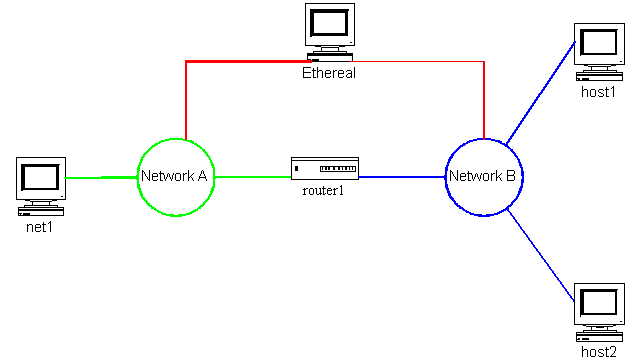
With these questions scrolling through your mind you decide to set up a little testbed and see what happens when these and other questions are implemented. Your setup consists of a machine you call net1, which connects to Network A. A full Policy Routing compliant system you call router1 is connected between this network and another network, Network B. On Network B host1 and host2 reside. You have an independent machine running Ethereal or any other packet capture utility you are familiar with that is connected to both networks so that you can see the details of the packets themselves. This setup is illustrated in Figure 6.1.1
This setup is the testbed you will use throughout this chapter as you explore advanced Policy Routing topics. The setup is quite flexible and may be added to easily.
Example 6.1.1 - The Art of Ping
To start your testing you set up the testing environment with the following addressing:
net1 192.168.1.1/24
router1 192.168.1.254/24
10.1.1.1/24
host1 10.1.1.2/24
host2 10.1.1.3/24
This setup defines Network A as 192.168.1.0/24 and Network B as 10.1.1.0/24. The two host machines have their default routes pointing at router1. The net1 machine only has a network route for 10.1.1.0/24 pointing at router1. And router1 has no default route set.
Under this set up, you can ping from net1 to all three devices, router1, host1, and host2. On the packet capture you can see that the arps are correctly answered on both sides of router1. This is traditional standard networking.
Now you want to see what happens if you start adding addresses to router1. First you try adding addresses to the physical interfaces on router1. You add 172.16.1.254/16 to the Network B interface of router1. Then you try pinging this interface from host1 and verify that is does respond. So router1 is routing between the two addresses on the single interface.
Now you decide to use a virtual interface on router1 to perform the same test. Looking through the list of available interfaces you decide to try the dummy interface set. On the system is a dummy0 interface which looks like the following:
[root@router1/root]# ip link ls dev dummy0
5: dummy0: <BROADCAST,NOARP> mtu 1500 qdisc noop
link/ether 00:00:00:00:00:00 brd ff:ff:ff:ff:ff:ff
Now you delete the 172.16.1.254/24 address from the Network B interface and add it to the dummy interface. Then you set the dummy interface active. Now your dummy0 interface looks as follows:
[root@router1/root]# ip addr ls dev dummy0
5: dummy0: <BROADCAST,NOARP,UP> mtu 1500 qdisc noqueue
link/ether 00:00:00:00:00:00 brd ff:ff:ff:ff:ff:ff
inet 172.16.1.254/24 scope global dummy0
inet6 fe80::200:ff:fe00:0/10 scope link
Finally you try pinging 172.16.1.254 from host1. The ping output looks exactly like the output from when you had assigned the address to the physical device interface. Now you see that the address is truly independent of the physical devices.
Curious, you look at the routing table on router1 to see if there is anything different about this setup:
[root@router1/root]# ip route ls
192.168.1.0/24 dev eth0 proto kernel scope link src 192.168.1.254
172.16.1.0/24 dev dummy0 proto kernel scope link src 172.16.1.254
10.1.1.0/24 dev eth1 proto kernel scope link src 10.1.1.254
Everything looks perfectly normal. Just for grins you try pinging 172.16.1.254 from the net1 machine. And you get the connect: Network is unreachable message response from net1. Of course net1 only has a route to the 10.1.1.0/24 network via router1 and has no route to the 172.16.1.0/24 network thus the ping packets never go anywhere.
Example 6.1.2 - Loopback Dummy
You think some more about how router1 can respond to the ping for 172.16.1.254 when the interface that contains the address is internal to the system itself. Indeed, you wonder how router1 responds to any type of ping. This leads to considering again how the Routing Policy Database (RPDB) works in this situation.
Considering how the system is responding you determine that since the address belongs to the system, then the system responds due to ownership. As you recall from reading through RFC-1122 this is the definition of a Weak ES host model (Section 3.3.4.2 - Multihoming Requirements) and thus is correct behaviour for any address owned by the system. The response follows the output procedures as specified through the RPDB. To consider the simple one-packet ping from host1 to router1 for the 172.16.1.254 address, you have the following simplified steps:
1. host1 checks its routing table and determines that it has no specific route to 172.16.1.254. Thus, it should send the packet to the default gateway, router1.
2. router1 receives the packet and determines that it owns the 172.16.1.254 address and so it should respond.
3. router1 consults its RPDB to determine the method of response. Since in this case there is a route with a provided source address it uses the src address to respond. Additionally, there is no defined route response so router1 responds using the local table route to host1.
4. host1 receives the response coded with the 172.16.1.254 source address.
Now statement 3 is deliberate in scope. The tangled logic is best illustrated by going through the following example. You really need to pay careful attention to the details to understand how the responses are generated.
First, you delete all addresses from dummy0 on router1 using the ip addr flush dev dummy0 command. Then you add back in the address to dev dummy0 using the host mask to prevent auto-route creation, ip addr add 172.16.1.254/32 dev dummy0. You then test this setup by pinging the address from host1 and note that you get a response.
Now you look at the routing table on router1. The route to 172.16.1.254 is coded only in the local table. This is as it should be because the local table contains all broadcast and interface routes. You note that this is the only location for this route. In other words there is no route referring to any network related to 172.16.1.254.
You create a table called table2, which refers to routing table 2, by adding a line to /etc/iproute2/rt_tables. Then you add a default route through net1 to table2, which specifies using the src of 172.16.1.254, ip route add default via 192.168.1.1 src 172.16.1.254 table table2.
So far you are not using this table, so a ping from host1 will still get a response. To use the table you create a rule. This rule is different and explained in just a bit:
ip rule add from 172.16.1.254 dev lo table 2 prio 2000
To ensure that this rule is used by the system immediately, you issue the ip route flush cache command.
Fire up the Ethereal capture on Network A and ping from host1 to 172.16.1.254. The capture looks like the following:
172.16.1.254 -> host2 ICMP Echo (ping) reply
172.16.1.254 -> host2 ICMP Echo (ping) reply
172.16.1.254 -> host2 ICMP Echo (ping) reply
172.16.1.254 -> host2 ICMP Echo (ping) reply
Note that you are listening on Network A, not on Network B where the ping originated from. The response packet was exactly as you suspected but sent to a different network. This is why the format of the rule statement is very important.
You dissect the rule statement by considering the actions in order. First, the rule is added with a from clause that specifies the address you added to dev dummy0, 172.16.1.254. This rule will look at all packets with source address 172.16.1.254. There is an additional qualifier, dev lo, that states that the interface through which the packet is originated must be lo, the loopback interface. But the interface to which the packet was supposedly destined and replied from is dummy0. This is the seemingly strange part.
You wonder if maybe this is due to dev dummy0 being somehow different from the physical interfaces. So you try the same sequence only this time you add the address to dev eth1, which is the Network B interface. All the rest of the commands are the same. And now when you ping, you get the same result.
What you see is that an address exists only to define a service - just as required by the tenets of Policy Routing. Yes, it seems weird to consider that an address assigned to a physical interface can be routed back through a different interface, but the really weird part is even thinking that the address is "assigned" to the interface. If you still think that this is strange behaviour read through both RFC-1122 and RFC-2101 very carefully.
At first glance this may seem to be a convoluted and theoretical example, but think back to asymmetric ("loopy") routing and consider the following setup.
Example 6.1.3 - Reality is Loopy
You have a Policy Routing firewall system, router1, similar to Example 5.2.3, "Troubleshooting Unbalanced Multiple Loop Routes," from Chapter 5. This system has three different interfaces defined on the system, as illustrated in Figure 6.1.3. The first interface, eth0, is connected to Network A, a legal IP network (real Internet routable addressing), provided through a 256K Frame connection. The second interface, eth1, is connected to Network B which has a connection to the Internet through a full T1 frame. The third interface, sat0, is connected to a high downlink speed satellite connection, which has a 64Kbps uplink and a 3Mbps downlink. The addressing is similar to the following (substituting private addresses):
eth0 192.168.1.254/24
gateway from Inet = 192.168.1.253/24
eth1 172.16.1.1/30
gateway to Inet = 172.16.1.2/30
sat0 10.1.1.1/30
gateway from/to Inet = 10.1.1.2/30
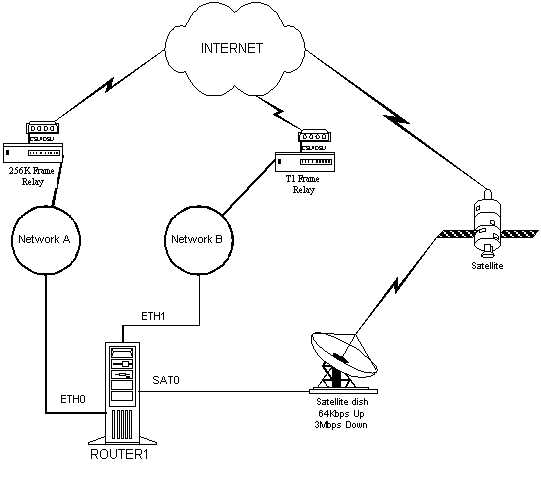
Figure 6.1.3 - Reality is Loopy
What you have is all of your Internet accessible devices on network 192.168.1.0/24. The default route for those devices is the router1 eth0 interface, 192.168.1.254. The uplink to the Internet for these devices is 172.16.1.2. This is so far just a simple example of assymetrical routing.
The router1 is also running named for DNS. This is a service being provided by router1 on all of its interfaces. Recalling how the outputs are seen from Example 6.1.2, you would think that there is only one way that the DNS server could be located. But you want DNS queries coming in the link from ISP #1, who provides the 256K link to go back out the 256K link with the address of eth0. Also, you want the DNS queries coming in from the link to ISP #2, the T1 provider, to return out that link with the address from eth1. Finally, you want DNS queries from the satellite link to go out the link to ISP #2 but using the sat0 address as source. Using the constructs from Example 6.1.2, this is easy.
You create a setup to handle these requirements. First you define three routing tables in /etc/iproute2/rt_tables. These are DMZ, Inet, and Sat. In each of these tables you place the following routes:
ip route add default via 192.168.1.253 table DMZ src 192.168.1.254
ip route add default via 172.16.1.2 table Inet src 172.16.1.1
ip route add default via 172.16.1.2 table Sat src 10.1.1.1
Now you define the rules to interact with these route tables. Note that in this case you only need deal with the source address because the incoming packet would already have been routed to the system.
ip rule add from 192.168.1.254 dev lo table DMZ prio 15000
ip rule add from 172.16.1.1 dev lo table Inet prio 15100
ip rule add from 10.1.1.1 dev lo table Sat prio 15200
Now you have your loopy routing and you get to DNS to.
All of these setups rely on the provision of addresses as independent from any physical definition. The address merely defines the location of a service.
There are times when being able to define the table to which you will send a packet is simply not enough. To this point you have specified usage of the RPDB that end in the final routing table destination. You wonder about additional interactions between the rules and route tables.
Returning to your test network setup you decide to make the two hosts, host1 and host2, appear as two different networks. To make the packet traces obvious, you use 172.16.1.1/24 for host2 and leave host1 on 10.1.1.3/24. On router1 you assign 10.1.1.254/24 and 172.16.1.254/24 to dev eth1 on Network B. After setting up these addresses you verify that host2 can ping all other systems.
So your test setup now has the following machines, addresses, and routes:
net1 192.168.1.1/24
No Default Route
Static route to 10.1.1.0/24 and 172.16.1.0/24 via router1
router1 eth0: 192.168.1.254/24 eth1: 10.1.1.254/24, 172.16.1.254/24
No additional routes
host1 10.1.1.1/24
Default route via 10.1.1.254
host2 172.16.1.1/24
Default route via 172.16.1.254
In order to see how the rules interact with the routing tables you first try a little experiment.
On host2 you add a few additional /32 addresses from the network, say 172.16.1.2-5. These will be the test addresses sending out data to see how the throw route works. You will use the traceroute utility to test using these extra addresses.
What you want to see is how the throw route can be used to bounce out of a routing table back to the rules. To this end on router1 you set up two tables. Each table has a default route pointing to a different router. Then you set up rules that take two of the extra addresses from host2 and send them to different tables. The command setup for this is as follows:
ip route add default via 10.1.1.2 src 10.1.1.254 table 2
ip route add default via 192.168.1.1 src 192.168.1.254 table 3
ip rule add from 172.16.1.2/32 table 2 prio 15000
ip rule add from 172.16.1.3/32 table 3 prio 15100
ip route flush cache
Now on host2 you issue two different traceroute commands to the same location using the two different addresses. The commands and output you get are as follows:
[root@host2/etc]# traceroute -s 172.16.1.2 192.168.1.1
traceroute to 192.168.1.1 (192.168.1.1) from 172.16.1.2, 30 hops max, 40 byte packets
1 router1 (10.1.1.254) 20.091 ms 0.566 ms 0.461 ms
2 * * *
(and so on)
[root@host2/etc]# traceroute -s 172.16.1.3 192.168.1.1
traceroute to 192.168.1.1 (192.168.1.1) from 172.16.1.3, 30 hops max, 40 byte packets
1 router1 (10.1.1.254) 0.976 ms 0.510 ms 0.458 ms
2 net1 (192.168.1.1) 0.700 ms 0.599 ms 0.576 ms
Just as you suspected, the traceroute that uses the 172.16.1.2 source address is sent into routing table 2 on router1. And that routing table contains a default route to host1. Host1 has no knowledge of the originating IP (172.16.1.2) and thus no return route so the probes just die off. You can see this in the packet trace on Network B where eventually an ICMP Destination Unreachable is sent back to 172.16.1.2. Unfortunately, in this case the traceroute program does not ever receive this message but you know that is a problem with the traceroute program itself.
Now you add a throw route to table 2 for the specific traceroute address destination. From Chapter 4 you know that the action of a throw route is to return from the routing table as though the routing lookup has failed. This throw route is added as follows:
ip route add throw 192.168.1.1/32 table 2
When you now retry the traceroute, it succeeds just like the other address did.
[root@host2/etc]# traceroute -s 172.16.1.2 192.168.1.1
traceroute to 192.168.1.1 (192.168.1.1) from 172.16.1.2, 30 hops max, 40 byte packets
1 router1 (10.1.1.254) 0.982 ms 0.610 ms 0.478 ms
2 net1 (192.168.1.1) 0.679 ms 0.623 ms 0.583 ms
What you logically deduce is that the throw route, being the best match in the routing table, is used for these packets. If you only had a single routing table, this action would have effectively terminated the routing and the packet would have been immediately returned unreachable. But due to the RPDB, the action instead is to evaluate the next rule in the list. In this case the next matching rule is the default rule 32766, which sends the lookup into table main. This table has a route to the destination and the lookup succeeds, with the result that the traceroute then succeeds.
At this point you may be asking yourself why you would ever want to use a throw route. After all, if the routing is set up correctly and Policy Routing is implemented, you should never need to use such a route.
Consider, then, the meshing of Example 6.1.3 with Example 6.2.1. What if you had a Web server that was running on a system with multiple addresses and multiple interfaces and routes. Most of the time you want this particular server to route each Web request via a different route depending on the address and interface.
For example, you know that the number one Web server in the Internet, Apache, can assign virtual hosts both to a single address and to multiple addresses. So say you had an Apache server that had two interfaces and each interface had three addresses. The Apache treats each of the six addresses as belonging to a different domain. Furthermore, you have several virtual servers on top of two of the addresses.
Here you are running ten virtual Web servers. Each of these servers has a different set of output files. All of the servers are required to be visible to the corporate network through a single router connection on one of the two networks. This router is specifically set up to only see one of the addresses assigned to the Web server. What you have on the server is a routing table for each address using the loopback rules as in Example 6.1.2 because each address gets routed through a different router.
You could add a specific route to the corporate network to each router table, but you know that corporate is considering different network schemes for that router and might also add other routers to other parts of the corporate network. In order to simplify your life when corporate changes their mind yet again, you decide to add throw routes to all of these tables for the corporate network. Then you create a new table containing the current routes to corporate and assign a rule after all the other rules that sends the traffic into that table. Now when corporate decides to add routers or change the existing router, you simply change the one table and everything continues to work.
By the way, that is a somewhat real example that I ended up implementing a few years back for a Web server that was both the corporate intranet server and the corporate Internet server. This setup is quite simple and easy to do and highly secure.
6.3 Tag Routing with TOS and fwmark (nfmark)
Of course using internal services and routing them differentially is great when you have access to a Policy Routing capable system. But most of the server systems running over IPv4 today do not implement much of the basic IPv4 suite, let alone the advanced networking portions. There are several facilities available to deal with these types of systems.
The first facility that comes to mind is the QoS (Quality of Service) umbrella of protocols. Many of the items within this scope were originally intended to provide very specific types of routing and queuing services. But what is more interesting, and relevant to this discussion, is the design as a whole.
When you consider most of the various items commonly lumped under the QoS umbrella, such as DiffServ, IntServ, or RSVP, you see that they were designed to prioritize packet traffic flows. A packet is classified and then queued and routed based on that classification. The important part to note is that the packet itself, in part or in whole, is used to make a classification decision about the packet - not unlike the decision made to route a packet based on source address.
This general view is true of all facets of Policy Routing. After all, Policy Routing is routing based on the entire packet itself. And, when you start to consider the actual realities of implementing a routing interface, you quickly realize that queuing is an integral part of the actual act of interfacing to the network thus the statement that QoS is an integral part of the scope of Policy Routing.
As with any large and complicated system, the various parts of Policy Routing as a whole have unique and specific roles that do not seem to be a part of the intent of the general system. Those roles of the QoS spectrum include traffic flow service levels and the various mechanisms for implementing the queuing structures, among others. That entire scope of usage would require another book and will not be discussed here.
The interesting part of the QoS family, in reference strictly to routing the packet, lies in the mechanisms for classification. As you learned in Chapter 3, one of the mechanisms for specifying a route within the RPDB is to use the TOS (Type of Service) tag within the packet header to select a route or drive a rule. Since almost all QoS classification mechanisms are designed to use this field, either in the original format or in various other methods (ref: DiffServ), these classification mechanisms can be used to select packets using very specific parameters.
The specification of the TOS field for use in Policy Routing is best made with a broadly scoped and yet very precise mechanism. Within the Linux implementation this description fits the classifier known as u32. The u32 classifier is a binary-based selection mechanism. It essentially uses two parameters to operate upon a packet. The first parameter is the binary offset into the packet, and the second parameter is the binary match. Because the offset is specified as a binary location, you can look at any given part of the packet. The binary match is specified as a pattern and a mask so that you can look for specific signature patterns or even very specific bits. Thus you have a comprehensive packet selection mechanism over the entire packet.
Packet selection mechanisms bring up the other facility of mention: packet filtering. Packet filtering mechanisms are usually considered a function of network security and control mechanisms. As with the QoS family, the essential nature of packet filtering is the important concept.
Packet filtering relies on the ability to select packets for perusal. Most of the packet filtering schemes use an internal representation of the selection mechanism to differentiate the packets. This selection mechanism representation usually takes the form of a tag field added to the packet during the period that the packet traverses the filtering device. Using the native tag field as a selector for routing provides the link to Policy Routing.
Within the Linux kernel, the packet filtering mechanisms ensconced during the 2.1 kernel development provide a mechanism for exposing this tag to the general networking structure. This is the fwmark, called nfmark in the NetFilter architecture. This mark is a specifically provided mapping from the internal tagging mechanism to the general network structures. The mark is administratively assigned as needed by a specific packet filter selection rule. This mark was in all of the 2.2 series kernels and was recently added into the new 2.3/2.4 series kernels.
Either of these two mechanisms, QoS classification or packet filter mark (fwmark & nfmark), allow you to specify a tag that decides the routing. These mechanisms can coexist within a single system and can even coexist with their original functionality. You get the best of both worlds.
The first of these two facilities you decide to examine is the firewall mark, fwmark. This facility exists in different but related implementations depending on which kernel you use. For the 2.1/2.2. series of kernels you would use the ipchains utility to fwmark the packet. For the 2.3/2.4 series you would use the iptables utility of NetFilter to provide the fwmark. You decide to check out both facilities because some of your older machines are running 2.2 kernels, while many of your newer test machines run the 2.4 series kernels.
Returning to your testing network setup you decide to install a 2.2.12 series kernel on router1 along with the ipchains utility. Then you set up a Web server on host2 along with three different addresses. You will use the fwmark facility of ipchains to tag packets entering router1 from net1. You will then use these tags to selectively allow access to specific addresses of host2.
The addresses assigned on host2 along with the Web aliases are as follows:
host2 10.1.1.3/24
web1 10.1.1.5/32
web2 10.1.1.6/32
web3 10.1.1.7/32
Now on the eth0 interface of router1 you will place your fwmark rules. Recall from Chapter 3 that the INPUT chain is where you would put your tagging rules. The FORWARD chain is after the RPDB along with the OUTPUT chain.
You decide for clarity that you will tag the inbound packets using a fwmark that is the same as the final octet of the destination address. So you implement the following set of chain rules on router1:
ipchains -A input -p tcp -s 0/0 -d 10.1.1.5 80 -m 5
ipchains -A input -p tcp -s 0/0 -d 10.1.1.6 80 -m 6
ipchains -A input -p tcp -s 0/0 -d 10.1.1.7 80 -m 7
This will tag any packets entering router1 from any interface that is destined for the host2 addresses. There are some additional specifications you can add to the ipchains command to further specify the interface and even the source. If you are interested in those features you know you can look them up in the man pages, but for now you only want to see how the fwmark tag works.
Now you set about using some rules to select routing tables for these fwmarked packets. You note that in the extended listing of the fwmark from ipchains using ipchains -L -n -v that the fwmark is coded as a hex value. Thus, you see that if you had used a fwmark of 10, the corresponding actual tag would be 0xa. With this in mind you set up the rules noting that the IP utility uses hex only in referring to the fwmark. You end up with the following set of rules:
ip rule add fwmark 5 table 5 prio 15000
ip rule add fwmark 6 table 6 prio 16000
ip rule add fwmark 7 table 7 prio 17000
Of course, you need to populate the tables with the appropriate routes. One of the features of this style of selection is that you can tag different types of packets with the same fwmark. So, for example, when implementing the chain rules on router1 you could have marked both 10.1.1.5 and 10.1.1.6 with the same fwmark. Then the rules will select tables based on this mark. Thus you can tie together disparate packet types into the same routing structure.
Now that you have tried out the fwmark facility in kernel 2.2.12, you decide to try kernel 2.4.0 on router1 and implement the same fwmark setup. Since you already know how the rules will look, you only need to figure out how to use the iptables utility under NetFilter. You come up with the following set of iptables commands that operate as the ipchains rules you set up on router1 operated. NOte that you have to specify these rules as operating on the mangle table as you are actually modifying the packet.
iptables -t mangle -A PREROUTING -p tcp -s 0/0 -d 10.1.1.5/32 --dport 80 -j MARK --set-mark 5
iptables -t mangle -A PREROUTING -p tcp -s 0/0 -d 10.1.1.6/32 --dport 80 -j MARK --set-mark 6
iptables -t mangle -A PREROUTING -p tcp -s 0/0 -d 10.1.1.7/32 --dport 80 -j MARK --set-mark 7
In Chapter 3 you learned that the NetFilter architecture allows you to specify two different locations for packet mangling operations. Since you want to see packets entering router1 from the network you choose the PREROUTING hook. The rules that act on this setup are the same as before.
Now both the ipchains and the iptables commands can be used to set marks within the OUTPUT hook location. This location sets the mark for packets that are exiting from the localhost or loopback interface. Thus you can use all of the dev lo rules you saw in Example 6.1.2 to route the marked packets.
6.4 Linux DiffServ Architecture
Now that you have tried out the packet filtering techniques for marking the packets, you decide to turn your attention to the QoS classification routines. These routines are designed to tag packets for use with queuing structures. These tags are often in the form of actual changes to the TOS field within the packet header.
To date, most implementations of QoS tend to implement classification and flow control on the output, called the egress, interface. This is purely due to the general viewpoint from the development time in the early 1990s that you were only performing traditional routing. Since in traditional routing a decision about the packet destination is not performed until just before the packet leaves the system, the general consensus was that any queuing must take place after the routing decision was made. The arrival of Policy Routing has revealed that this idea, as with the traditional routing structure, is limited.
Fortunately, the Linux DiffServ architecture provides an ingress (input) queuing discipline that can meet your needs. This ingress queuing discipline (qdisc) is currently only capable of tagging and policing packets on the ingress. But the plans and future hopes are that it will grow to become a regular full-function qdisc. Additionally, there is an idea floating around to associate the entire DiffServ architecture on Linux with the services rather than the physical interface, similar in thought to the way an address within Policy Routing belongs to a service and not a physical device. Since the entire structure of QoS, including DiffServ, is considered a part of the full Policy Routing structure, this move would align all network mechanisms in the same generalized structure. And that would be best all the way around.
To use the ingress qdisc you need to understand a little of the DiffServ architecture with respect to the various terms and mechanics. In a nutshell, the qdisc is the core function that provides a method for queuing the packets. The class is the group into which the packet is placed and by which the qdisc is selective of packets. The filter is attached to the qdisc and is the selector of the packet. Basically you enable a qdisc, attach filters to the qdisc, and provide classes within the qdisc. For your purposes the actual classification will be done by the filter because the filter is the tagging mechanism.
There is a difference between a queue and a queuing discipline. Each particular network device has a queue that feeds packets to it. Within that device queue you may have several queuing disciplines at work. Think of a store where there is only one register at which you actually purchase your item and leave the store. That register is the device queue. From that register there are several lines that start within the store at a single point, and branch out into several lines that then converge again on the single register. Think of the entire system, beginning with the single entry point into the lines and ending at the single register, as the device queue itself. Then the various lines represent various possible queuing disciplines.
For the ingress qdisc you need only consider that there is only one possible line. Hopefully when the newer generalized structures are implemented, perhaps in 2.5 series Linux development kernels, there will be more possible lines to choose from.
Queuing disciplines and classes are fundamentally intertwined. A queuing discipline may contain several classes of service. These classes and their semantics are fundamental properties of that queuing discipline. Thinking again of the store register lines, each originating line within the whole queue can be a class of the queuing discipline. Each class can contain other queuing disciplines within it, which then can contain classes, and so on and so on. In the end all of the machinations serve merely to differentiate the service received by the various packets.
A queuing discipline does not necessarily have classes. For example, the TBF queuing discipline (see Glossary) does not allow classes. If you use TBF you essentially have a single overall class for the entire queuing discipline. In the ingress qdisc there is no real need for classes because the current function is only to provide a mechanism for tagging a packet on reception.
Filters provide the method for checking and tagging packets. These tags can then be used by the classes to determine the membership in the class. Filters may be combined arbitrarily with queuing disciplines. Thinking again about the store analogy, the point where a single line splits into several parallel lines indicates the location of a filter application. The actual split mechanism could be a class decision based on an earlier filter tag. Consider the case where everybody who has less than five items and wants to pay cash will be put into the "less than five items & pays cash" line. There is a filter entity that checks each person and if they are a "less than 5 & cash," they are given a tag. Either then or later on another entity, think of class or RPDB, moves the person to another line based on the tag.
Now that you have an idea of how the basic set up works within the Linux DiffServ mechanism, you decide to play with using the ingress qdisc for routing tags.
In order to test this model you decide to use the 2.4 kernel with the classid-to-mark DiffServ extension. This extension will be part of the regular DiffServ code within the 2.4 series kernels. It provides an internal conversion map between a classid tag from a filter to a fwmark. In this way you can use the ultimate packet tagging power tool, the u32 classifier.
You go to router1 and make sure it is running a 2.4 kernel without any of the NetFilter architecture turned on. Then you set up the ingress qdisc on the Network B interface, eth1:
tc qdisc add dev eth1 handle ffff: ingress
Now you need to consider how the u32 filter works.
The most powerful filter available in Linux is the u32 filter. This filter allows you to actually make a choice based on any data within the packet itself. As with all of the DiffServ implementation for Linux you will use the tc utility from IPROUTE2. In this book the complete syntax and use of the tc utility will not be covered, Please refer to the IPROUTE2 documentation for details. Looking at the tc utility help for this filter gives a faint glimpse of this power:
tc filter add u32 help
Usage: ... u32 [ match SELECTOR ... ] [ link HTID ] [ classid CLASSID ]
[ police POLICE_SPEC ] [ offset OFFSET_SPEC]
[ ht HTID ] [ hashkey HASHKEY_SPEC ]
[ sample SAMPLE ] or u32 divisor DIVISOR
Where: SELECTOR := SAMPLE SAMPLE ...
SAMPLE := { ip | ip6 | udp | tcp | icmp | u{32|16|8} } SAMPLE_ARGS
FILTERID := X:Y:Z
The actual heavy-duty selection mechanisms are in the SELECTOR. But all you are told is that the SELECTOR is a series of SAMPLE sections. And nowhere are you told what the SAMPLE_ARGS would have to be. But by reading through the source and looking around the Internet you amass some of the needed information for using u32 in the context of this book.
The u32 selectors are simply binary patterns with binary masks that are used to match any set of data within the packet. The most common usage is to perform matches within the packet header. There are two main types of selectors that are deeply interrelated. The human interface selectors are those that are specified using linguistic aliases for the actions specifying specific protocol and field matches, such as the IP destination address or protocol 4. Then there are the bitwizard selectors that are specified in terms of the bit pattern length. These selectors are the u32, u16, and u8 selectors themselves. Within the tc utility all of the human selectors are translated into bitwizard selectors.
For example, if you specify matching the human selector "match ip tos 0x10 0xff," the tc utility actually matches against the packet as "match u8 0x10 0xff at 1." Note from the human specification that you are trying to match TOS 10h. Now the TOS field within an IP header is one byte long, which is 8 bits and thus a u8 general length selector, and located at a one byte offset into the IP packet. Thus you can specify matching a one byte set of bits with a full mask located at one byte into the packet header, which is "match u8 0x10 0xff at 1." Or you can say "match ip tos 0x10 0xff."
Now you can see why this is bitwizard work. There is no man page or other help, you have to know your packet binary structure and hexadecimal conversions, and even the human interface is somewhat cryptic. But the power available using this filter is incredible. The ability to specify any binary data pattern means that you can pick out individual data streams for routing. Suppose that you are browsing several different Web sites from your machine. To the router, all the data streams look as though they originate from the same address to the same protocol. By using u32, you could look for data patterns that indicate SSL encryption on either the sent or returned packets and route them through a secure link. And that is without looking at the header at all.
Additionally, you can look for certain types of patterns by using the mask portion of the specification. In the TOS example from the previous paragraph you were looking for exactly TOS 16 decimal, which is 0x10 hex. But what if you wanted to consider all TOS decimal levels from 16 through 19 inclusive? You would just change the mask portion of the specification and would then have a command like match u8 0x10 0xf3 at 1. Thus between the specification of the length of pattern, the pattern itself, and the offset into the packet you can isolate any unique portion of the packet. You can also stack several selectors together to obtain any combination of selections you require.
As you work with the u32 filter you note some tricky behaviors on the part of the selectors. You consider the filter snippet match tcp src 0x1234. This human filter is coded by tc as match u16 0x1234 0xffff nexthdr+0, which means to match a 16-bit 0x1234 pattern within the internal protocol header at offset 0. But what is contained within the offset 0 of the internal protocol header is simply the IPv4 source port for the packet.
Thus, if you were expecting the match tcp part to only match TCP packets, you would be surprised. The filter snippet will actually match UDP packets as well because they also have the source port contained at offset 0 within the internal protocol header. If you want to specify only matching TCP packets with source port 0x1234, then you have to stack up selectors. You would then use match tcp src 0x1234 match ip protocol 0x6. The additional selector match ip protocol 0x6 states to also only look at packets of protocol 6 hex, which is TCP. Here is the list of u32 selectors as known at this time. Be sure to read through RFC-791 and RFC-1122 for details about the IPv4 Header field definitions.
match <ip,tcp,udp> src <ip source address/mask CIDR>
match <ip.tcp,udp> dst <ip destination address/mask CIDR>
match ip tos <original 5bit IPv4 TOS field in hex> <hex mask>
match ip dsfield <entire 8bit IPv4 TOS field> <hex mask>
match ip precedence <original 3bit precedemce section of TOS field> <hex mask>
match ip ihl <8 bit ip header length in hex>
match ip protocol <ip protocol number in hex> <hex mask>
match ip nofrag = only match non fragmented ip packets
match ip firstfrag = only match first ip fragment
match ip df = IP Data Fragments (ie: !firstfrag ??)
match ip mf = Matching Fragments (related to ??)
match <ip,tcp,udp> sport <source port in hex> <hex mask>
match <ip,tcp,udp> dport <dest port in hex> <hex mask>
match ip icmp_type <icmp type in hex> <hex mask>
match ip icmp_code <icmp code in hex> <hex mask>
match icmp type <icmp type in hex> <hex mask>
match icmp code <icmp code in hex> <hex mask>
As you can see there are many ways in which you can look into the packet headers and determine your selection. When you combine these facilities with the ability to also specify any exact bit pattern at any offset into the packet that you want, you can see the power of the Linux DiffServ architecture.
Within the u32 filter there is another kind of selector available, the sample command. The sample command takes the same kinds of arguments as match. However, the sample command normally takes only a single argument for type. So where you would use match ip protocol 0x6 0xff, you can use sample tcp instead.
With your newly acquired knowledge of the u32 filter usage you first decide to try a simple test of the ingress filter. You know you have the ingress qdisc set up on router1 on the Network B interface. You decide to try tagging all incoming packets from 10.1.1.0/24 with classid 1. Then you will use a rule that sends those packets into table 1 and assign them additionally to realms 3/4 for tracking. You end up with the following sequence of commands:
tc filter add dev eth1 parent ffff: protocol ip prio 1 u32 \
match ip src 10.1.1.0/24 classid :1
ip rule add fwmark 1 table 1 prio 15000 realms 3/4
ip route add default via 192.168.1.1 table 1 src 192.168.1.254
ip route flush cache
Then you run a ping from net1 to host1 and look at the output of the qdisc statistics and the realms:
[root@router1 /root]# tc -s qdisc ls dev eth1
qdisc ingress ffff: ----------------
Sent 0 bytes 0 pkts (dropped 0, overlimits 0)
[root@router1 /root]# rtacct 3
Realm BytesTo PktsTo BytesFrom PktsFrom
3 0 0 504 6
[root@router1 /root]# rtacct 4
Realm BytesTo PktsTo BytesFrom PktsFrom
4 504 6 0 0
You note that the qdisc statistics do not show any traffic. That is expected because you are not using the classid anywhere on egress for DiffServ. You are only using the ingress qdisc to be able to tag packets with the u32 filter. You know that the filter is working because you have your ping packets showing up balanced on the realms. The only way the realms would list the packets is if they were acted upon by that rule. So your quick test was successful.
6.5 Interactions with Packet Filters
In your testing of the u32 qdisc you came to wonder what interactions exist between the NetFilter mangle and the u32 filter. You know from testing the fwmark that the mangle table can select and mark packets on input using the PREROUTING hook. You know from your u32 testing that the u32 filter can select and mark packets on ingress. Does one override the other or can they coexist?
Example 6.5.1 - Double Play Packet
You decide to try a quick test now that you have seen good examples of both types of packet tagging. You have router1 set up with a 2.4 kernel and both the NetFilter and the DiffServ running. You then run the following set of commands to set up the tagging mechanisms for both iptables and u32:
tc qdisc add dev eth1 handle ffff: ingress
tc filter add dev eth1 parent ffff: protocol ip prio 1 u32 \
match ip src 10.1.1.0/24 classid :2
iptables -t mangle -i eth1 -A PREROUTING -s 10.1.1.0/24 -d 0/0 -j MARK --set-mark 1
ip rule add fwmark 1 table 1 prio 15000 realms 1/2
ip rule add fwmark 2 table 2 prio 15100 realms 3/4
ip route add default via 192.168.1.1 src 192.168.1.254 table 1
ip route add default via 192.168.1.1 src 192.168.1.254 table 2
Now you try a ping from net1 to host2 and look at your realms. The only ones with any traffic are realms 1/2:
[root@router1 /root]# rtacct
Realm BytesTo PktsTo BytesFrom PktsFrom
1 0 0 336 4
2 336 4 0 0
[root@router1 /root]# rtacct 3
Realm BytesTo PktsTo BytesFrom PktsFrom
3 0 0 0 0
[root@router1 /root]# rtacct 4
Realm BytesTo PktsTo BytesFrom PktsFrom
3 0 0 0 0
You know that the rtacct utility will only list out the realms that have actual counts in them. Just to make sure, you manually listed realm 3 and realm 4 and found them empty.
Now you do wonder if maybe the fact that the rule for the u32 filter was of a higher priority, 15000, than the rule for NetFilter, 15100. So just to make sure you reverse the order of the commands, change the priorities on the rules, reboot router1, and try again. Your command listing looks like this:
iptables -t mangle -i eth1 -A PREROUTING -s 10.1.1.0/24 -d 0/0 -j MARK --set-mark 1
tc qdisc add dev eth1 handle ffff: ingress
tc filter add dev eth1 parent ffff: protocol ip prio 1 u32 \
match ip src 10.1.1.0/24 classid :2
ip rule add fwmark 2 table 2 prio 15000 realms 3/4
ip rule add fwmark 1 table 1 prio 15100 realms 1/2
ip route add default via 192.168.1.1 src 192.168.1.254 table 1
ip route add default via 192.168.1.1 src 192.168.1.254 table 2
You try this setup and it gives the exact same output as the first. So you correctly conclude that the NetFilter framework operates at a lower level within the packet tagging structures than the ingress qdisc, and that the one does not override the other.
Now you decide quickly to test out the coexistence. To this end you set up the following script, which uses u32 to tag host1 and iptables to mark host2:
iptables -t mangle -i eth1 -A PREROUTING -s 10.1.1.3/32 -d 0/0 -j MARK --set-mark 2
tc qdisc add dev eth1 handle ffff: ingress
tc filter add dev eth1 parent ffff: protocol ip prio 1 u32 \
match ip src 10.1.1.2/32 classid :1
ip rule add fwmark 2 table 2 prio 15000 realms 3/4
ip rule add fwmark 1 table 1 prio 15100 realms 1/2
ip route add default via 192.168.1.1 src 192.168.1.254 table 1
ip route add default via 192.168.1.1 src 192.168.1.254 table 2
When you run this script you get output for all four realms. Recalling that earlier the two tagging mechanisms were set to tag the same packets, you realize that you can now have the best of both worlds. The NetFilter mark can be used on the packet headers and the u32 classifier can be used on arbitrary binary data from the packet. This allows for a truly powerful system.
What you have learned are some of the deeper workings of the usage of Policy Routing. The actions of any single part of the system are uniquely consistent across all scales. You have seen how the basic principles extend consistently to more complicated problems. When the problem is broken down into the components and their needs, the setup of the system is simple logic.
The inconsistencies are found not from within Policy Routing but from the preconceptions and interactions with other systems. As in the finest arts, a thorough understanding of the basic mechanisms produce the finest products when combined.
You look forward to implementing and extending your structure to the rest of your networks. First you want to conquer the dynamic routing setups already present within your network and deal with the need under IPv4 to change your addressing. Then you wonder how the new IPv6 structures work within these contexts. To those and other goals you set your sights.
Return to Table of Contents